Antenna Setup
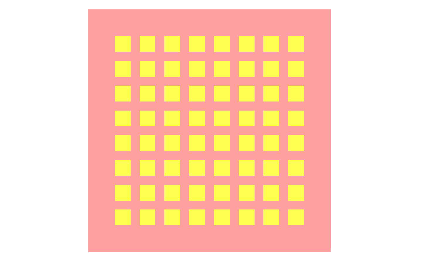
Figure 1: A top view of the antenna geometry showing the layout of the 8x8 array of patches.
The antenna geometry consists of a 52.5 x 52.5 mm sheet of dielectric material (dielectric constant = 2.2, loss tangent 0.0009, thickness 0.254 mm) that is backed by a conducting ground plane and topped with 64 patch elements in an 8x8 configuration. Each patch is 3.4025 mm square and is spaced a half-wavelength at 28 GHz (approximately 5.36 mm) apart. A view of the patch layout on the dielectric sheet is visible in Figure 1. The feed point for each antenna is offset from the center of the patch by 0.75 mm in the horizontal direction as this was found to be the location of the best return loss result. A 28 GHz sinusoidal waveform is used at each patch with an adjustable phase offset that is determined based on the desired direction of the main beam. A widely-used formula for determining the phasing of the elements for a beam focused at a direction of θd, φd is
Wn = exp{-j(2π/λ) sin(θd)[ xn cos(φd) + yn sin(φd)]}
where xn and yn are the locations (in meters) of the feeds at each patch referenced to the initial patch in the lower left corner of the array, and w n is the phase shift for the element located at (xn, yn). In XFdtd, these phases were assigned to each feed element through the use of parameters as shown in Figure 2, where the phase shift is defined by a parameter name.

Figure 2: An example of one of the source definitions for the patch feeds, showing the phase shift set as a variable which may be adjusted depending on the desired beam direction.
Results
Simulations were performed on the array to determine the gain pattern possible for different phasing conditions. An initial test set all phases equal so all elements are radiating toward the (0°, 0°) direction. This resulted in a maximum gain of just over 23 dBi and a 3 dB beamwidth of just over 12 degrees as shown in a line plot through one of the principal planes in Figure 3. The same pattern is shown over the CAD drawing of the antenna in three dimensions in Figure 4. With the phases adjusted to direct a beam toward (20°, 90°) the result is a slight drop in peak gain to 22.9 dBi and a broadening of the beamwidth to about 13.2 degrees, shown in three dimensions in Figure 5. Sweeping the beam to a corner of the array at direction (45°, 40°) reduces the peak gain down to 21.7 dBi and broadens the beam a moderate amount (Figure 6). As the phasing is changed to steer the beam toward the horizon, the array reaches a limit due to the patterns of the original patch antennas, and a gain plot with large side lobes forms. In Figure 7 several beam patterns are shown together to illustrate the steering of the beam from normal down to 50 degrees in 10-degree steps.
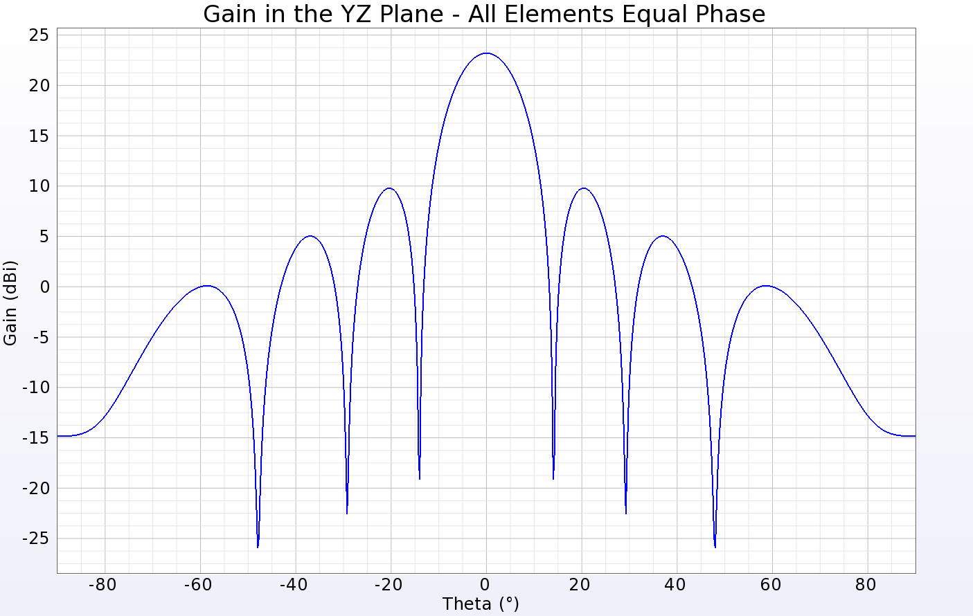
Figure 3: A line plot of the gain in a cross-sectional cut of the array pattern for the case where all patches are fed in-phase with equal amplitudes. The peak gain is just over 23 dBi and the 3 dB beamwidth is about 12 degrees.
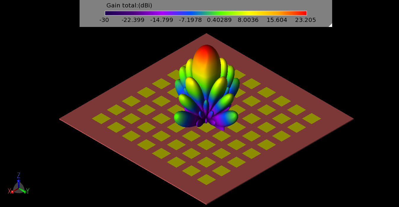
Figure 4: The three-dimensional gain pattern for the 8x8 array when all patches are fed in-phase with equal amplitudes.
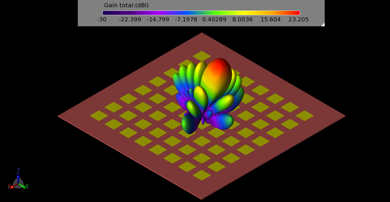
Figure 5: The three-dimensional gain pattern for the 8x8 array when the patches are phased to direct the main beam toward (20°, 90°).
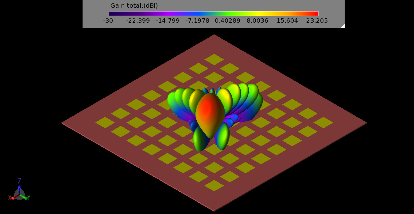
Figure 6: The three-dimensional gain pattern for the 8x8 array when the patches are phased to direct the main beam toward (40°, 45°).
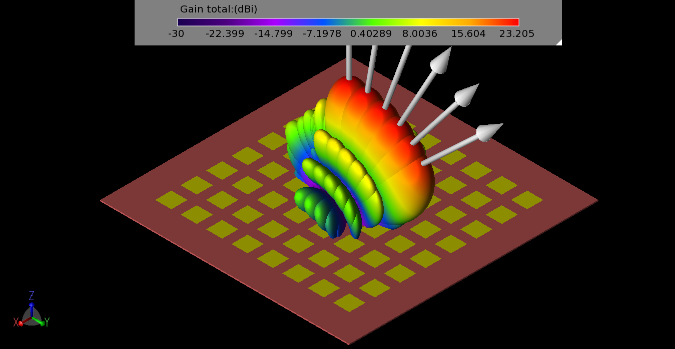
Figure 7: Three-dimensional gain patterns for six gain patterns from the 8x8 array for phasing set to direct the beam to (0°,90°) to (50°, 90°) in 10-degree increments.
Simulations for return loss were run for each port and were found to have values below -30 dB indicating the patches were properly tuned. Radiation efficiency varied from about 78% up to more than 90% over the array, with patches near the edges of the array generally having higher efficiencies.
To examine the performance of sub-arrays, a few simple cases were simulated to find typical results for 4x4, 2x2, and 1x2 arrays of elements. All these simulations were performed with the patches fed with equal phase signals. The patterns for 4x4 and 2x2 sub-arrays in a corner of the main array are shown in Figure 8 and Figure 9. Two locations on the array, one near an edge and one near the center, were simulated as 1x2 sub-arrays and there were only minor differences in their results. A typical pattern for a 1x2 sub-array defined near the center of the main array is shown in Figure 10.
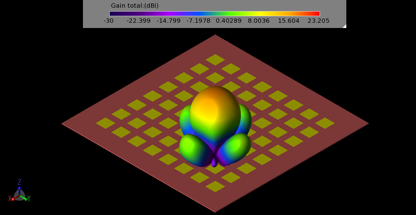
Figure 8: The three-dimensional gain pattern for a 4x4 sub-array of elements in one quadrant of the main array.
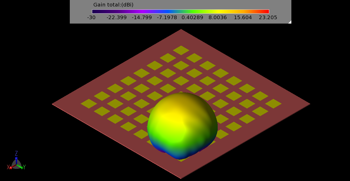
Figure 9: The three-dimensional gain pattern for a 2x2 sub-array of elements in one corner of the main array.
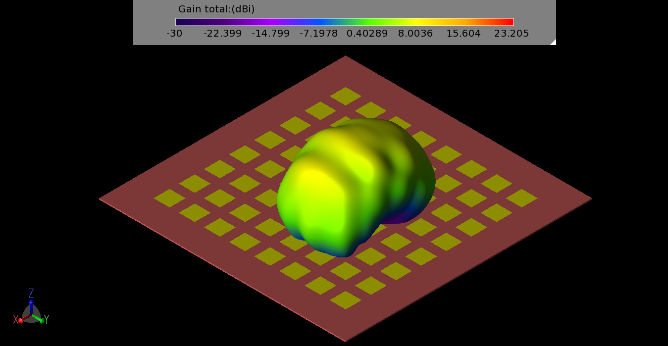
Figure 10: The three-dimensional gain pattern for a 1x2 sub-array of elements near the center of the main array.
It is inefficient to simulate all possible phasing combinations to determine the overall performance of the array. However, a macro program in XFdtd is available that allows a full examination of the gain levels at all angles from the array by sweeping the phasing of the individual elements. The result is a plot showing the cumulative distribution function (CDF) of the effective isotropic radiated power (EIRP). The EIRP is an indication of the power an antenna can radiate in a given direction compared to an isotropic radiator. This plot may be used to determine the fractional area of the far-zone sphere that has gain above 0 dBi for a given input power level. Generally speaking, a power level of 23 dBmW is used as the input level for mobile devices. When the CDF for the entire 8x8 array is generated, it is found that the 23 dBmW level is about 0.225 fractional area (Figure 11), meaning that (1 – 0.225 = 0.775) 77.5% of the far-zone sphere can be illuminated with gain above 0 dBi. The 4x4 sub-array (Figure 12) has 64.3% coverage at 23 dBmW input power. Similar plots are shown for the 2x2 sub-array (Figure 13, 50%), and a 1x2 sub-array near the center of the main array (Figure 14, 40.2%). Many other sub-arrays beyond those shown here are possible and may be of value depending on the needs of the system.
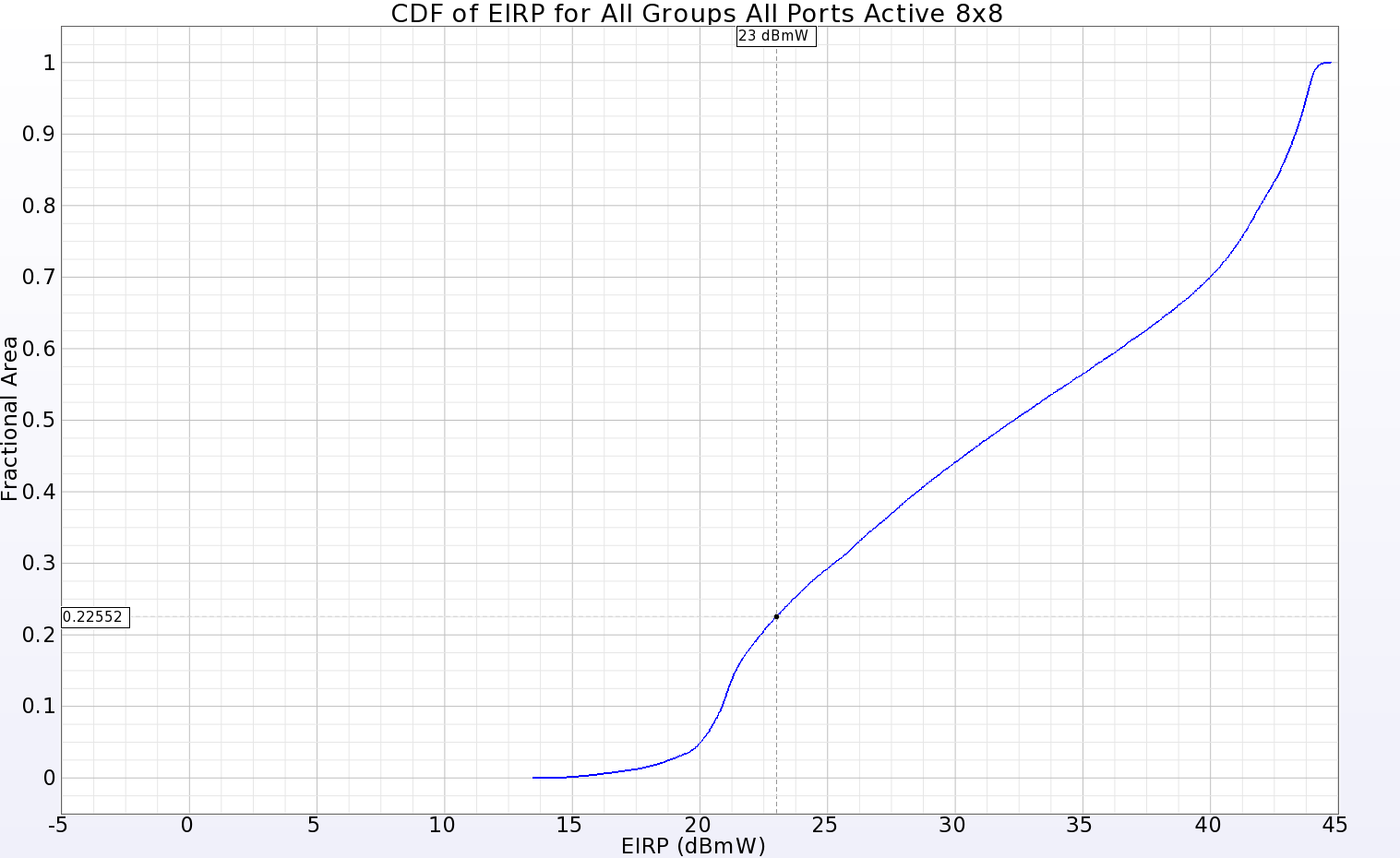
Figure 11: The CDF of EIRP plot for the full 8x8 array shows positive gain over 77.5% of the far-zone sphere for an input power of 23 dBmW.
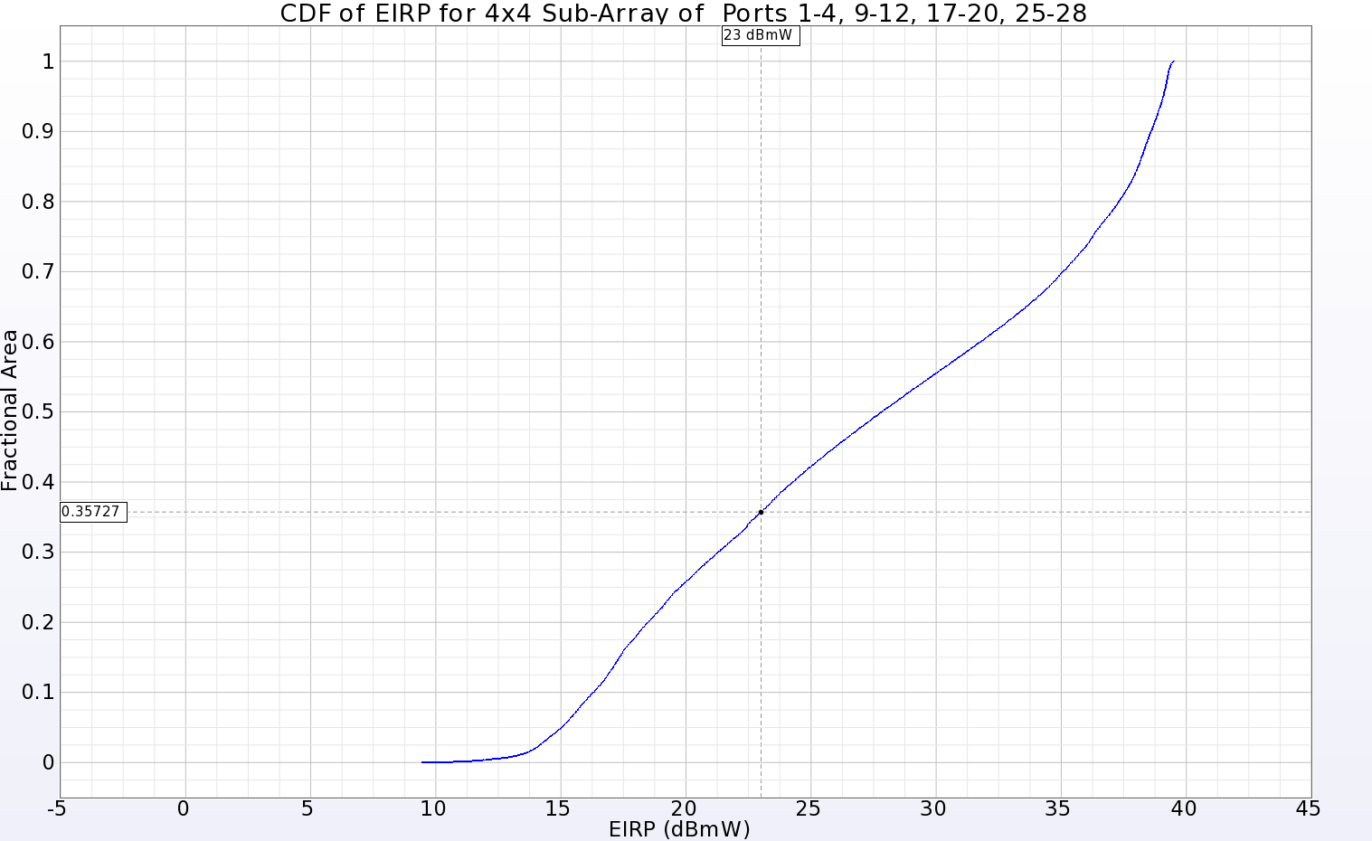
Figure 12: The CDF of EIRP plot for a 4x4 sub-array located in one quadrant of the main array showing positive gain over 64.3% of the far-zone sphere for an input power of 23 dBmW.
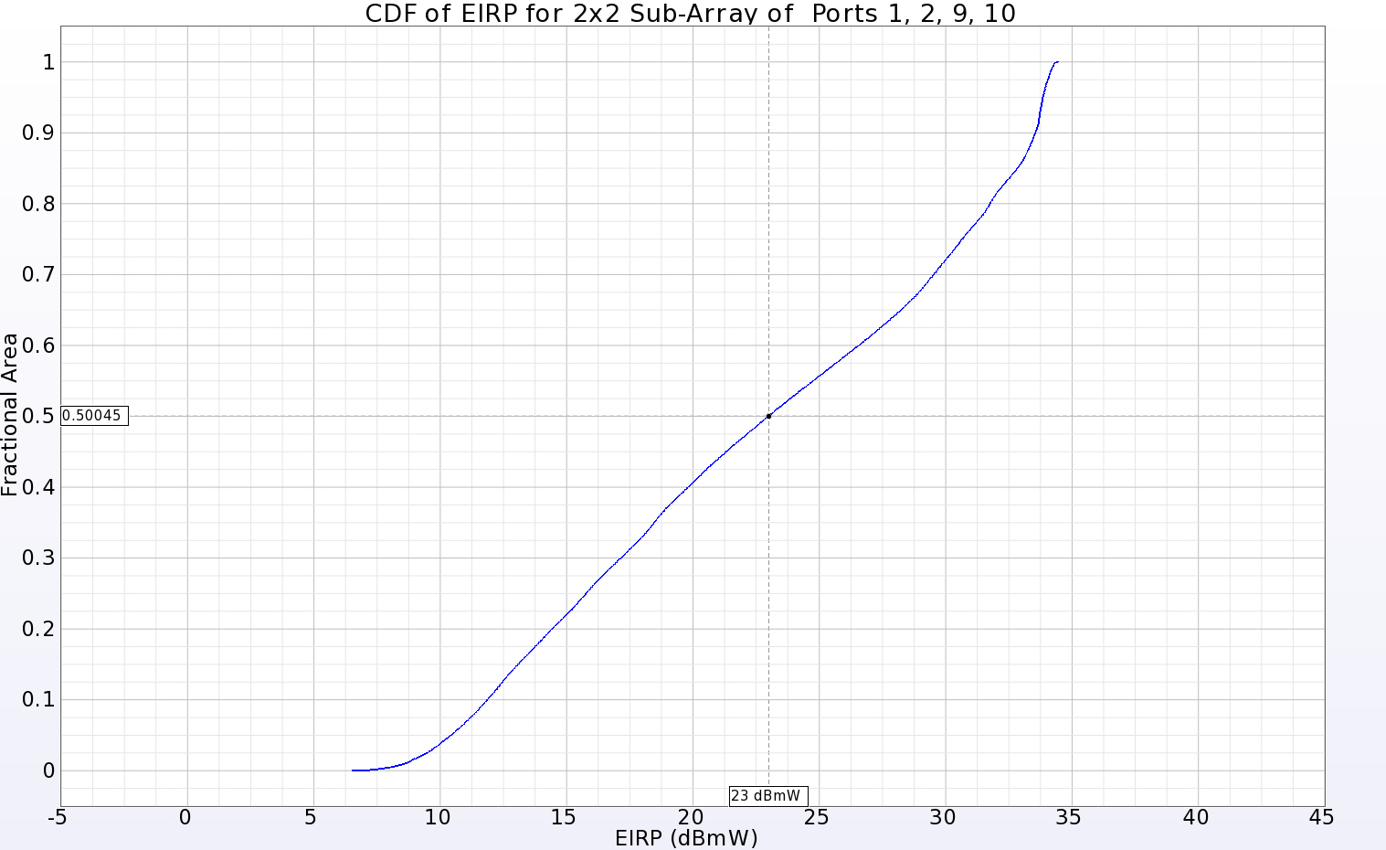
Figure 13: The CDF of EIRP plot for a 2x2 sub-array located in one corner of the main array showing positive gain over 50% of the far-zone sphere for an input power of 23 dBmW.
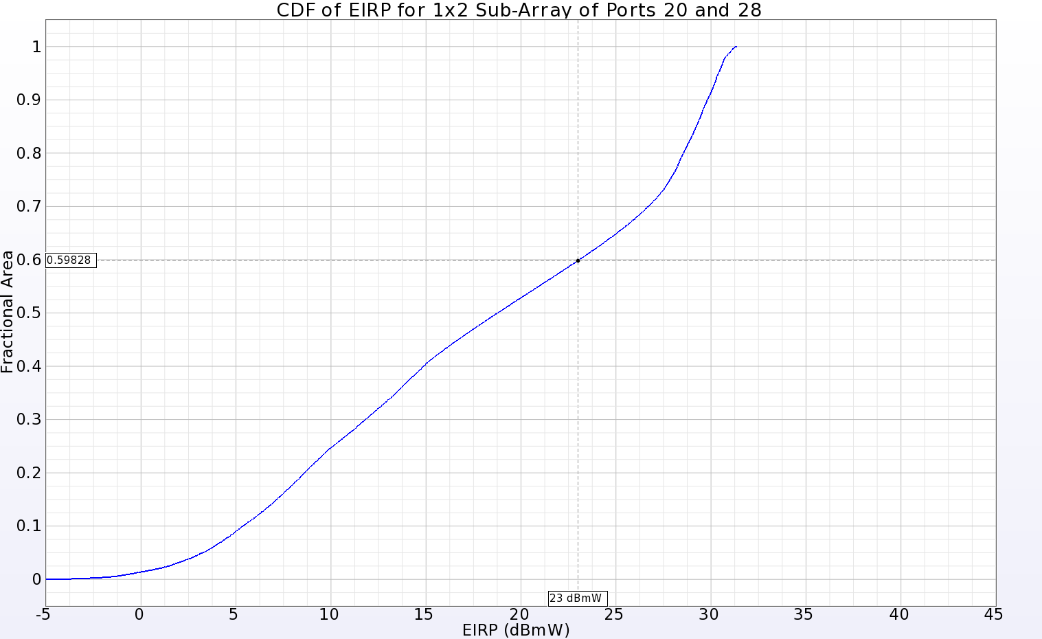
Figure 14: The CDF of EIRP plot for a 1x2 sub-array located in near the center of the main array showing positive gain over 40.2% of the far-zone sphere for an input power of 23 dBmW.